Modeling Antennas

Under Development

Too see plots run in google colab: https://colab.research.google.com/github/casangi/sirius/blob/main/docs/antenna_beams.ipynb

Load Packages

import os
try:
    import sirius
    print('SiRIUS version',sirius.__version__,'already installed.')
except ImportError as e:
    print(e)
    print('Installing SiRIUS')
    os.system("pip install sirius")
    import sirius
    print('SiRIUS version',sirius.__version__,' installed.')

import pkg_resources
import xarray as xr
import numpy as np
from ipywidgets import interactive, fixed
from sirius.display_tools import display_J, display_M
from sirius.calc_beam import make_mueler_mat

from astropy.coordinates import SkyCoord
xr.set_options(display_style="html")
import os
try:
    from google.colab import output
    output.enable_custom_widget_manager()
    IN_COLAB = True
except:
    IN_COLAB = False
%matplotlib widget
#%matplotlib inline

SiRIUS version 0.0.22 already installed.

Voltage Pattern and Primary Beam

The Voltage Pattern (VP) is the image plane response of a single antenna and the Primary Beam (PB) is the image plane response of pair of antennas (baselines) and is given by:

\[PB = VP \odot VP^*\]

where \(^*\) is the complex conjugate and \(\odot\) is the Hadamard product (element wise product).

\(^T\) transpose. \(^H\) Hermitian or complex conjugate transpose.

Aperture illumination function (AIP)

from sirius.calc_beam import calc_beam, calc_zpc_beam
import numpy as np
from sirius_data.beam_1d_func_models.airy_disk import aca, alma, vla
print(vla)

#freq_chan = np.array([60*10**9,90*10**9,100*10**9,120*10**9])
freq_chan = np.array([90*10**9])
#freq_chan = np.array([3.052*10**9])
beam_parms = {}
J_xds = calc_beam(alma,freq_chan,beam_parms,check_parms=True)
#J_xds = calc_beam(vla,freq_chan,beam_parms,check_parms=True)
J_xds

{'func': 'casa_airy', 'dish_diam': 24.5, 'blockage_diam': 0.0, 'max_rad_1GHz': 0.014946999714079439}
Setting default fov_scaling  to  4.0
Setting default mueller_selection  to  [ 0  5 10 15]
Setting default zernike_freq_interp  to  nearest
Setting default pa_radius  to  0.2
Setting default image_size  to  [1000 1000]
[1000 1000] [-1.38385217e-06  1.38385217e-06] 4.0 0.03113667385557884

<xarray.Dataset>
Dimensions:  (chan: 1, pa: 1, pol: 1, l: 1000, m: 1000)
Coordinates:
  * chan     (chan) int64 90000000000
  * pa       (pa) int64 0
  * pol      (pol) int64 0
  * l        (l) float64 0.0006919 0.0006905 0.0006892 ... -0.0006892 -0.0006905
  * m        (m) float64 -0.0006919 -0.0006905 ... 0.0006892 0.0006905
Data variables:
    J        (pa, chan, pol, l, m) float64 0.01527 0.01577 ... 0.0168 0.0163

xarray.Dataset

• Dimensions:
  • chan: 1
  • pa: 1
  • pol: 1
  • l: 1000
  • m: 1000
• Coordinates: (5)
  • chan
    (chan)
    int64
    90000000000

    array([90000000000])

  • pa
    (pa)
    int64
    0

    array([0])

  • pol
    (pol)
    int64
    0

    array([0])

  • l
    (l)
    float64
    0.0006919 0.0006905 ... -0.0006905

    array([ 0.000692,  0.000691,  0.000689, ..., -0.000688, -0.000689, -0.000691])

  • m
    (m)
    float64
    -0.0006919 -0.0006905 ... 0.0006905

    array([-0.000692, -0.000691, -0.000689, ...,  0.000688,  0.000689,  0.000691])

• Data variables: (1)
  • J
    (pa, chan, pol, l, m)
    float64
    0.01527 0.01577 ... 0.0168 0.0163

    array([[[[[0.01527003, 0.01577455, 0.01629718, ..., 0.01680182,
               0.01629718, 0.01577455],
              [0.01577455, 0.01629718, 0.01680182, ..., 0.01730645,
               0.01680182, 0.01629718],
              [0.01629718, 0.01680182, 0.01730645, ..., 0.01781102,
               0.01730645, 0.01680182],
              ...,
              [0.01680182, 0.01730645, 0.01781102, ..., 0.01833349,
               0.01781102, 0.01730645],
              [0.01629718, 0.01680182, 0.01730645, ..., 0.01781102,
               0.01730645, 0.01680182],
              [0.01577455, 0.01629718, 0.01680182, ..., 0.01730645,
               0.01680182, 0.01629718]]]]])

• Attributes: (0)

from sirius.display_tools import display_J

interactive_plot_1 = interactive(display_J, J_xds=fixed(J_xds), pa=fixed(0), chan=(0,J_xds.dims['chan']-1), val_type=['abs','phase','real','imag'],units=['rad','arcsec','arcmin','deg'])
output_1 = interactive_plot_1.children[-1]
output_1.layout.auto_scroll_threshold = 9999;
interactive_plot_1

EVLA Polynomial Model

%load_ext autoreload
%autoreload 2

pc_dir = pkg_resources.resource_filename('sirius_data', 'beam_polynomial_coefficient_models/data/EVLA_.bpc.zarr')
pc_xds = xr.open_zarr(pc_dir,consolidated=False)

pc_xds = pc_xds.where(pc_xds.band=='S',drop=True)
#pc_xds = pc_xds.isel(chan=[36,37])
print(pc_xds.band.values)
print(pc_xds.chan.values)
pc_xds

['S' 'S' 'S' 'S' 'S' 'S' 'S' 'S' 'S' 'S' 'S' 'S' 'S' 'S' 'S']
[2.052e+09 2.180e+09 2.436e+09 2.564e+09 2.692e+09 2.820e+09 2.948e+09
 3.052e+09 3.180e+09 3.308e+09 3.436e+09 3.564e+09 3.692e+09 3.820e+09
 3.948e+09]

<xarray.Dataset>
Dimensions:    (chan: 15, pol: 1, coef_indx: 5)
Coordinates:
    band       (chan) <U1 dask.array<chunksize=(15,), meta=np.ndarray>
  * chan       (chan) float64 2.052e+09 2.18e+09 ... 3.82e+09 3.948e+09
  * coef_indx  (coef_indx) int64 0 1 2 3 4
  * pol        (pol) int64 5
Data variables:
    BPC        (chan, pol, coef_indx) float64 dask.array<chunksize=(15, 1, 5), meta=np.ndarray>
    ETA        (chan, pol, coef_indx) float64 dask.array<chunksize=(15, 1, 5), meta=np.ndarray>
Attributes:
    conversion_date:  2022-01-27
    dish_diam:        25
    max_rad_1GHz:     0.014946999714079439
    pc_file_name:     EVLA_.txt
    telescope_name:   EVLA

xarray.Dataset

• Dimensions:
  • chan: 15
  • pol: 1
  • coef_indx: 5
• Coordinates: (4)
  • band
    (chan)
    <U1
    dask.array<chunksize=(15,), meta=np.ndarray>

    Array Chunk Bytes 60 B 60 B Shape (15,) (15,) Count 4 Tasks 1 Chunks Type numpy.ndarray

  • chan
    (chan)
    float64
    2.052e+09 2.18e+09 ... 3.948e+09

    array([2.052e+09, 2.180e+09, 2.436e+09, 2.564e+09, 2.692e+09, 2.820e+09,
           2.948e+09, 3.052e+09, 3.180e+09, 3.308e+09, 3.436e+09, 3.564e+09,
           3.692e+09, 3.820e+09, 3.948e+09])

  • coef_indx
    (coef_indx)
    int64
    0 1 2 3 4

    array([0, 1, 2, 3, 4])

  • pol
    (pol)
    int64
    5

    array([5])

• Data variables: (2)
  • BPC
    (chan, pol, coef_indx)
    float64
    dask.array<chunksize=(15, 1, 5), meta=np.ndarray>

    Array Chunk Bytes 600 B 600 B Shape (15, 1, 5) (15, 1, 5) Count 11 Tasks 1 Chunks Type float64 numpy.ndarray

  • ETA
    (chan, pol, coef_indx)
    float64
    dask.array<chunksize=(15, 1, 5), meta=np.ndarray>

    Array Chunk Bytes 600 B 600 B Shape (15, 1, 5) (15, 1, 5) Count 11 Tasks 1 Chunks Type float64 numpy.ndarray

• Attributes: (5)

  conversion_date :

  2022-01-27

  dish_diam :

  25

  max_rad_1GHz :

  0.014946999714079439

  pc_file_name :

  EVLA_.txt

  telescope_name :

  EVLA

from sirius.calc_beam import calc_bpc_beam

J_xds = calc_bpc_beam(pc_xds,pc_xds.chan.values,beam_parms={})
J_xds

Setting default fov_scaling  to  4.0
Setting default mueller_selection  to  [ 0  5 10 15]
Setting default zernike_freq_interp  to  nearest
Setting default pa_radius  to  0.2
Setting default image_size  to  [1000 1000]
cell_size  [-2.91364517e-05  2.91364517e-05]

<xarray.Dataset>
Dimensions:  (chan: 15, pa: 1, pol: 1, l: 1000, m: 1000)
Coordinates:
  * chan     (chan) float64 2.052e+09 2.18e+09 2.436e+09 ... 3.82e+09 3.948e+09
  * pa       (pa) int64 0
  * pol      (pol) int64 0
  * l        (l) float64 0.01457 0.01454 0.01451 ... -0.01448 -0.01451 -0.01454
  * m        (m) float64 -0.01457 -0.01454 -0.01451 ... 0.01448 0.01451 0.01454
Data variables:
    J        (pa, chan, pol, l, m) float64 0.0 0.0 0.0 0.0 ... 0.0 0.0 0.0 0.0

xarray.Dataset

• Dimensions:
  • chan: 15
  • pa: 1
  • pol: 1
  • l: 1000
  • m: 1000
• Coordinates: (5)
  • chan
    (chan)
    float64
    2.052e+09 2.18e+09 ... 3.948e+09

    array([2.052e+09, 2.180e+09, 2.436e+09, 2.564e+09, 2.692e+09, 2.820e+09,
           2.948e+09, 3.052e+09, 3.180e+09, 3.308e+09, 3.436e+09, 3.564e+09,
           3.692e+09, 3.820e+09, 3.948e+09])

  • pa
    (pa)
    int64
    0

    array([0])

  • pol
    (pol)
    int64
    0

    array([0])

  • l
    (l)
    float64
    0.01457 0.01454 ... -0.01454

    array([ 0.014568,  0.014539,  0.01451 , ..., -0.014481, -0.01451 , -0.014539])

  • m
    (m)
    float64
    -0.01457 -0.01454 ... 0.01454

    array([-0.014568, -0.014539, -0.01451 , ...,  0.014481,  0.01451 ,  0.014539])

• Data variables: (1)
  • J
    (pa, chan, pol, l, m)
    float64
    0.0 0.0 0.0 0.0 ... 0.0 0.0 0.0 0.0

    array([[[[[0., 0., 0., ..., 0., 0., 0.],
              [0., 0., 0., ..., 0., 0., 0.],
              [0., 0., 0., ..., 0., 0., 0.],
              ...,
              [0., 0., 0., ..., 0., 0., 0.],
              [0., 0., 0., ..., 0., 0., 0.],
              [0., 0., 0., ..., 0., 0., 0.]]],
    
    
            [[[0., 0., 0., ..., 0., 0., 0.],
              [0., 0., 0., ..., 0., 0., 0.],
              [0., 0., 0., ..., 0., 0., 0.],
              ...,
              [0., 0., 0., ..., 0., 0., 0.],
              [0., 0., 0., ..., 0., 0., 0.],
              [0., 0., 0., ..., 0., 0., 0.]]],
    
    
            [[[0., 0., 0., ..., 0., 0., 0.],
              [0., 0., 0., ..., 0., 0., 0.],
    ...
              [0., 0., 0., ..., 0., 0., 0.],
              [0., 0., 0., ..., 0., 0., 0.]]],
    
    
            [[[0., 0., 0., ..., 0., 0., 0.],
              [0., 0., 0., ..., 0., 0., 0.],
              [0., 0., 0., ..., 0., 0., 0.],
              ...,
              [0., 0., 0., ..., 0., 0., 0.],
              [0., 0., 0., ..., 0., 0., 0.],
              [0., 0., 0., ..., 0., 0., 0.]]],
    
    
            [[[0., 0., 0., ..., 0., 0., 0.],
              [0., 0., 0., ..., 0., 0., 0.],
              [0., 0., 0., ..., 0., 0., 0.],
              ...,
              [0., 0., 0., ..., 0., 0., 0.],
              [0., 0., 0., ..., 0., 0., 0.],
              [0., 0., 0., ..., 0., 0., 0.]]]]])

• Attributes: (0)

from sirius.display_tools import display_J

interactive_plot_1 = interactive(display_J, J_xds=fixed(J_xds), pa=fixed(0), chan=(0,J_xds.dims['chan']-1), val_type=['abs','phase','real','imag'],units=['rad','arcsec','arcmin','deg'])
output_1 = interactive_plot_1.children[-1]
output_1.layout.auto_scroll_threshold = 9999;
interactive_plot_1

Jones Matrix

Sky Jones matrix as a function of direction is given by

\[\begin{split}\textbf{J}_i^{sky} (\textbf{s}) = \begin{bmatrix} J^p_i & -J^{p \rightarrow q}_i \\ J_i^{q \rightarrow p} & J^{q}_i \end{bmatrix}\end{split}\]

Simplified case of the Airy disk (real valued and symmetric)

\[\begin{split}\textbf{J}_i^{sky} (\textbf{s}) = \begin{bmatrix} J^p_i & 0 \\ 0 & J^{p}_i \end{bmatrix}\end{split}\]

No leakage and p=q.

SiRIUS stores Jones matrices row wise

\[\begin{split}\begin{bmatrix} 0 & 1 \\ 2 & 3 \end{bmatrix}\end{split}\]

import pkg_resources

zpc_dir = pkg_resources.resource_filename('sirius_data', 'aperture_polynomial_coefficient_models/data/EVLA_avg_zcoeffs_SBand_lookup.apc.zarr')
zpc_xds = xr.open_zarr(zpc_dir,consolidated=False)
freq_chan = zpc_xds.chan.values#np.array([2.1*10**9,2.4*10**9,2.8*10**9,3.4*10**9])

zpc_xds

<xarray.Dataset>
Dimensions:    (chan: 16, pol: 4, coef_indx: 66)
Coordinates:
  * chan       (chan) float64 2.052e+09 2.18e+09 ... 3.844e+09 3.972e+09
  * coef_indx  (coef_indx) int64 0 1 2 3 4 5 6 7 8 ... 58 59 60 61 62 63 64 65
  * pol        (pol) int64 5 6 7 8
Data variables:
    ETA        (chan, pol, coef_indx) float64 dask.array<chunksize=(16, 4, 66), meta=np.ndarray>
    ZPC        (chan, pol, coef_indx) complex128 dask.array<chunksize=(16, 4, 66), meta=np.ndarray>
Attributes:
    apc_file_name:    EVLA_avg_zcoeffs_SBand_lookup.csv
    conversion_date:  2022-01-27
    dish_diam:        25
    max_rad_1GHz:     0.014946999714079439
    telescope_name:   EVLA

xarray.Dataset

• Dimensions:
  • chan: 16
  • pol: 4
  • coef_indx: 66
• Coordinates: (3)
  • chan
    (chan)
    float64
    2.052e+09 2.18e+09 ... 3.972e+09

    array([2.052e+09, 2.180e+09, 2.308e+09, 2.436e+09, 2.564e+09, 2.692e+09,
           2.820e+09, 2.948e+09, 3.076e+09, 3.204e+09, 3.332e+09, 3.460e+09,
           3.588e+09, 3.716e+09, 3.844e+09, 3.972e+09])

  • coef_indx
    (coef_indx)
    int64
    0 1 2 3 4 5 6 ... 60 61 62 63 64 65

    array([ 0,  1,  2,  3,  4,  5,  6,  7,  8,  9, 10, 11, 12, 13, 14, 15, 16, 17,
           18, 19, 20, 21, 22, 23, 24, 25, 26, 27, 28, 29, 30, 31, 32, 33, 34, 35,
           36, 37, 38, 39, 40, 41, 42, 43, 44, 45, 46, 47, 48, 49, 50, 51, 52, 53,
           54, 55, 56, 57, 58, 59, 60, 61, 62, 63, 64, 65])

  • pol
    (pol)
    int64
    5 6 7 8

    array([5, 6, 7, 8])

• Data variables: (2)
  • ETA
    (chan, pol, coef_indx)
    float64
    dask.array<chunksize=(16, 4, 66), meta=np.ndarray>

    Array Chunk Bytes 33.00 kiB 33.00 kiB Shape (16, 4, 66) (16, 4, 66) Count 2 Tasks 1 Chunks Type float64 numpy.ndarray

  • ZPC
    (chan, pol, coef_indx)
    complex128
    dask.array<chunksize=(16, 4, 66), meta=np.ndarray>

    Array Chunk Bytes 66.00 kiB 66.00 kiB Shape (16, 4, 66) (16, 4, 66) Count 2 Tasks 1 Chunks Type complex128 numpy.ndarray

• Attributes: (5)

  apc_file_name :

  EVLA_avg_zcoeffs_SBand_lookup.csv

  conversion_date :

  2022-01-27

  dish_diam :

  25

  max_rad_1GHz :

  0.014946999714079439

  telescope_name :

  EVLA

beam_parms={}
beam_parms['mueller_selection'] = np.arange(16)
J_xds_zpc = calc_zpc_beam(zpc_xds,np.array([0,np.pi/4,np.pi*2/4,np.pi*3/4,np.pi]),freq_chan,beam_parms)
J_xds_zpc

Setting default fov_scaling  to  4.0
Setting default zernike_freq_interp  to  nearest
Setting default pa_radius  to  0.2
Setting default image_size  to  [1000 1000]

<xarray.Dataset>
Dimensions:  (chan: 16, pa: 5, pol: 4, l: 1000, m: 1000)
Coordinates:
  * chan     (chan) float64 2.052e+09 2.18e+09 2.308e+09 ... 3.844e+09 3.972e+09
  * pa       (pa) float64 0.0 0.7854 1.571 2.356 3.142
  * pol      (pol) int64 5 6 7 8
  * l        (l) float64 0.01457 0.01454 0.01451 ... -0.01448 -0.01451 -0.01454
  * m        (m) float64 -0.01457 -0.01454 -0.01451 ... 0.01448 0.01451 0.01454
Data variables:
    J        (pa, chan, pol, l, m) complex128 (-0.12695041266544269-0.0096647...

xarray.Dataset

• Dimensions:
  • chan: 16
  • pa: 5
  • pol: 4
  • l: 1000
  • m: 1000
• Coordinates: (5)
  • chan
    (chan)
    float64
    2.052e+09 2.18e+09 ... 3.972e+09

    array([2.052e+09, 2.180e+09, 2.308e+09, 2.436e+09, 2.564e+09, 2.692e+09,
           2.820e+09, 2.948e+09, 3.076e+09, 3.204e+09, 3.332e+09, 3.460e+09,
           3.588e+09, 3.716e+09, 3.844e+09, 3.972e+09])

  • pa
    (pa)
    float64
    0.0 0.7854 1.571 2.356 3.142

    array([0.      , 0.785398, 1.570796, 2.356194, 3.141593])

  • pol
    (pol)
    int64
    5 6 7 8

    array([5, 6, 7, 8])

  • l
    (l)
    float64
    0.01457 0.01454 ... -0.01454

    array([ 0.014568,  0.014539,  0.01451 , ..., -0.014481, -0.01451 , -0.014539])

  • m
    (m)
    float64
    -0.01457 -0.01454 ... 0.01454

    array([-0.014568, -0.014539, -0.01451 , ...,  0.014481,  0.01451 ,  0.014539])

• Data variables: (1)
  • J
    (pa, chan, pol, l, m)
    complex128
    (-0.12695041266544269-0.00966477...

    array([[[[[-1.26950413e-01-9.66477674e-03j,
               -1.26888486e-01-9.65811699e-03j,
               -1.26809320e-01-9.65163706e-03j, ...,
               -1.27032724e-01-9.68582414e-03j,
               -1.27022533e-01-9.67863144e-03j,
               -1.26995096e-01-9.67161525e-03j],
              [-1.27019567e-01-9.66042232e-03j,
               -1.26957725e-01-9.65379039e-03j,
               -1.26878637e-01-9.64733922e-03j, ...,
               -1.27101572e-01-9.68139191e-03j,
               -1.27091492e-01-9.67422420e-03j,
               -1.27064157e-01-9.66723396e-03j],
              [-1.27071099e-01-9.65602276e-03j,
               -1.27009346e-01-9.64941950e-03j,
               -1.26930341e-01-9.64299788e-03j, ...,
               -1.27152797e-01-9.67691168e-03j,
               -1.27142825e-01-9.66976997e-03j,
               -1.27115593e-01-9.66280661e-03j],
              ...,
              [-1.26637312e-01-9.67756820e-03j,
    ...
                4.44606705e-02+1.17779263e-03j],
              ...,
              [ 4.43368583e-02+1.21123067e-03j,
                4.43132062e-02+1.18876656e-03j,
                4.42662946e-02+1.16645278e-03j, ...,
                4.42680216e-02+1.27935983e-03j,
                4.43142762e-02+1.25654405e-03j,
                4.43372206e-02+1.23382871e-03j],
              [ 4.44079012e-02+1.20053840e-03j,
                4.43842227e-02+1.17797880e-03j,
                4.43372598e-02+1.15557180e-03j, ...,
                4.43389955e-02+1.26896724e-03j,
                4.43852977e-02+1.24604942e-03j,
                4.44082652e-02+1.22323417e-03j],
              [ 4.44557746e-02+1.18953535e-03j,
                4.44320637e-02+1.16688468e-03j,
                4.43850526e-02+1.14438858e-03j, ...,
                4.43868716e-02+1.25824869e-03j,
                4.44331886e-02+1.23523421e-03j,
                4.44561551e-02+1.21232411e-03j]]]]])

• Attributes: (0)

interactive_plot_1 = interactive(display_J, J_xds=fixed(J_xds_zpc), pa=(0,J_xds_zpc.dims['pa']-1), chan=(0,J_xds_zpc.dims['chan']-1), val_type=['abs','phase','real','imag'],units=['rad','arcsec','arcmin','deg'])
output_1 = interactive_plot_1.children[-1]
output_1.layout.auto_scroll_threshold = 9999;
interactive_plot_1

Mueller Matrix

\[\textbf{M}^{sky}_{ij}(\textbf{s}) = \textbf{J}_i^{sky}(\textbf{s}) \otimes \textbf{J}_j^{sky}(\textbf{s})\]

SiRIUS stores Jones matrices row wise

\[\begin{split}\begin{bmatrix} 0 & 1 & 2 & 3 \\ 4 & 5 & 6 & 7 \\ 8 & 9 & 10 & 11 \\ 12 & 13 & 14 & 15 \end{bmatrix}\end{split}\]

#Het array support
#make_mueler_mat(J_xds1, J_xds2, mueller_selection)

M_xds = make_mueler_mat(J_xds_zpc,J_xds_zpc,beam_parms['mueller_selection']) #np.array([ 0, 5, 10, 15])
M_xds

(5, 16, 4, 1000, 1000) (5, 16, 4, 1000, 1000)

<xarray.Dataset>
Dimensions:  (chan: 16, pa: 5, m_sel: 16, l: 1000, m: 1000)
Coordinates:
  * chan     (chan) float64 2.052e+09 2.18e+09 2.308e+09 ... 3.844e+09 3.972e+09
  * pa       (pa) float64 0.0 0.7854 1.571 2.356 3.142
  * m_sel    (m_sel) int64 0 1 2 3 4 5 6 7 8 9 10 11 12 13 14 15
  * l        (l) float64 0.01457 0.01454 0.01451 ... -0.01448 -0.01451 -0.01454
  * m        (m) float64 -0.01457 -0.01454 -0.01451 ... 0.01448 0.01451 0.01454
    pol1     (m_sel) float64 5.0 5.0 6.0 6.0 5.0 5.0 ... 8.0 8.0 7.0 7.0 8.0 8.0
    pol2     (m_sel) float64 5.0 6.0 5.0 6.0 7.0 8.0 ... 5.0 6.0 7.0 8.0 7.0 8.0
Data variables:
    M        (pa, chan, m_sel, l, m) complex128 (0.01620981518531084+0j) ... ...

xarray.Dataset

• Dimensions:
  • chan: 16
  • pa: 5
  • m_sel: 16
  • l: 1000
  • m: 1000
• Coordinates: (7)
  • chan
    (chan)
    float64
    2.052e+09 2.18e+09 ... 3.972e+09

    array([2.052e+09, 2.180e+09, 2.308e+09, 2.436e+09, 2.564e+09, 2.692e+09,
           2.820e+09, 2.948e+09, 3.076e+09, 3.204e+09, 3.332e+09, 3.460e+09,
           3.588e+09, 3.716e+09, 3.844e+09, 3.972e+09])

  • pa
    (pa)
    float64
    0.0 0.7854 1.571 2.356 3.142

    array([0.      , 0.785398, 1.570796, 2.356194, 3.141593])

  • m_sel
    (m_sel)
    int64
    0 1 2 3 4 5 6 ... 10 11 12 13 14 15

    array([ 0,  1,  2,  3,  4,  5,  6,  7,  8,  9, 10, 11, 12, 13, 14, 15])

  • l
    (l)
    float64
    0.01457 0.01454 ... -0.01454

    array([ 0.014568,  0.014539,  0.01451 , ..., -0.014481, -0.01451 , -0.014539])

  • m
    (m)
    float64
    -0.01457 -0.01454 ... 0.01454

    array([-0.014568, -0.014539, -0.01451 , ...,  0.014481,  0.01451 ,  0.014539])

  • pol1
    (m_sel)
    float64
    5.0 5.0 6.0 6.0 ... 7.0 7.0 8.0 8.0

    array([5., 5., 6., 6., 5., 5., 6., 6., 7., 7., 8., 8., 7., 7., 8., 8.])

  • pol2
    (m_sel)
    float64
    5.0 6.0 5.0 6.0 ... 7.0 8.0 7.0 8.0

    array([5., 6., 5., 6., 7., 8., 7., 8., 5., 6., 5., 6., 7., 8., 7., 8.])

• Data variables: (1)
  • M
    (pa, chan, m_sel, l, m)
    complex128
    (0.01620981518531084+0j) ... (0....

    array([[[[[ 1.62098152e-02+0.00000000e+00j,
                1.61939670e-02+0.00000000e+00j,
                1.61737578e-02+0.00000000e+00j, ...,
                1.62311282e-02+0.00000000e+00j,
                1.62283999e-02+0.00000000e+00j,
                1.62212946e-02+0.00000000e+00j],
              [ 1.62272942e-02+0.00000000e+00j,
                1.62114597e-02+0.00000000e+00j,
                1.61912597e-02+0.00000000e+00j, ...,
                1.62485390e-02+0.00000000e+00j,
                1.62458380e-02+0.00000000e+00j,
                1.62387554e-02+0.00000000e+00j],
              [ 1.62403029e-02+0.00000000e+00j,
                1.62244853e-02+0.00000000e+00j,
                1.62042988e-02+0.00000000e+00j, ...,
                1.62614763e-02+0.00000000e+00j,
                1.62588025e-02+0.00000000e+00j,
                1.62517438e-02+0.00000000e+00j],
              ...,
              [ 1.61306640e-02+0.00000000e+00j,
    ...
                1.97813841e-03+0.00000000e+00j],
              ...,
              [ 1.96722408e-03+0.00000000e+00j,
                1.96507341e-03+0.00000000e+00j,
                1.96086545e-03+0.00000000e+00j, ...,
                1.96129450e-03+0.00000000e+00j,
                1.96533398e-03+0.00000000e+00j,
                1.96731146e-03+0.00000000e+00j],
              [ 1.97350298e-03+0.00000000e+00j,
                1.97134685e-03+0.00000000e+00j,
                1.96712795e-03+0.00000000e+00j, ...,
                1.96755680e-03+0.00000000e+00j,
                1.97160729e-03+0.00000000e+00j,
                1.97359032e-03+0.00000000e+00j],
              [ 1.97773089e-03+0.00000000e+00j,
                1.97556990e-03+0.00000000e+00j,
                1.97134252e-03+0.00000000e+00j, ...,
                1.97177756e-03+0.00000000e+00j,
                1.97583405e-03+0.00000000e+00j,
                1.97781946e-03+0.00000000e+00j]]]]])

• Attributes: (0)

interactive_plot_1 = interactive(display_M, M_xds=fixed(M_xds), pa=(0,J_xds_zpc.dims['pa']-1), chan=(0,J_xds_zpc.dims['chan']-1), val_type=['abs','phase','real','imag'],units=['rad','arcsec','arcmin','deg'])
output_1 = interactive_plot_1.children[-1]
output_1.layout.auto_scroll_threshold = 9999;
interactive_plot_1

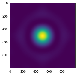
import matplotlib.pyplot as plt
plt.figure()
plt.imshow(np.real(M_xds.M[0,0,0,:,:]))
plt.show()

%load_ext autoreload
%autoreload 2

The autoreload extension is already loaded. To reload it, use:
  %reload_ext autoreload